Detection and Classification of pieces in a real Chess Board

🔗 GitHub Repository

This project was done as my Final Degree Project for the University of Málaga. The purpose of this project is to develop a neural network system that detects and classifies chess pieces on a real board, outputting their positions in FEN format. It uses a custom-labeled dataset and applies deep learning and computer vision techniques to ensure accurate performance under varying lighting conditions. The system aims to help digitize physical chess games for enthusiasts.

📖 You can read my Final Degree Project paper in this Linkedin Post.

---

🔍 Project Overview

This project focuses on automating the recognition of chessboard positions using YOLOv8, OpenCV, and a custom dataset. The output is provided in Forsyth-Edwards Notation (FEN) for seamless import into platforms like Lichess.

• Built for chess players, streamers, and tournament digitization
• Generates both annotated images and FEN strings
• Evaluated under variable lighting and angles

---

🎯 Goals

🎯 General Goal

Develop software that detects and classifies chess pieces on a real board image and outputs FEN.

✅ Specific Objectives

• Create a labeled dataset from real board photos.
• Train a deep learning model to detect/classify pieces.
• Detect the board grid via computer vision techniques.
• Map pieces to cells and produce FEN.
• Evaluate accuracy under different lighting and rotations.

---

🛠 Technologies Used

Category	Tools
Language	Python
Deep Learning	YOLOv8 (Ultralytics)
Data Labeling	CVAT
Vision Processing	OpenCV
Experiments	Google Colab
Data Analysis	Pandas, Matplotlib, SciPy
IDE / Tooling	Visual Studio Code, Git & GitHub

---

📷 Dataset Creation

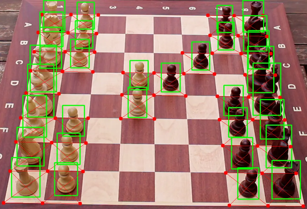
Due to the lack of publicly available datasets that suited the specific needs of my project, I decided to create my own. I used a camera to capture images of a chessboard placed in my yard, ensuring a variety of natural lighting conditions. Each image was then meticulously labeled manually, identifying every piece individually.

Dataset Features

The resulting dataset has the following characteristics:

• 130 labeled images from video frames (Canon EOS100D)
• Uniform angle (side-right view) for consistency
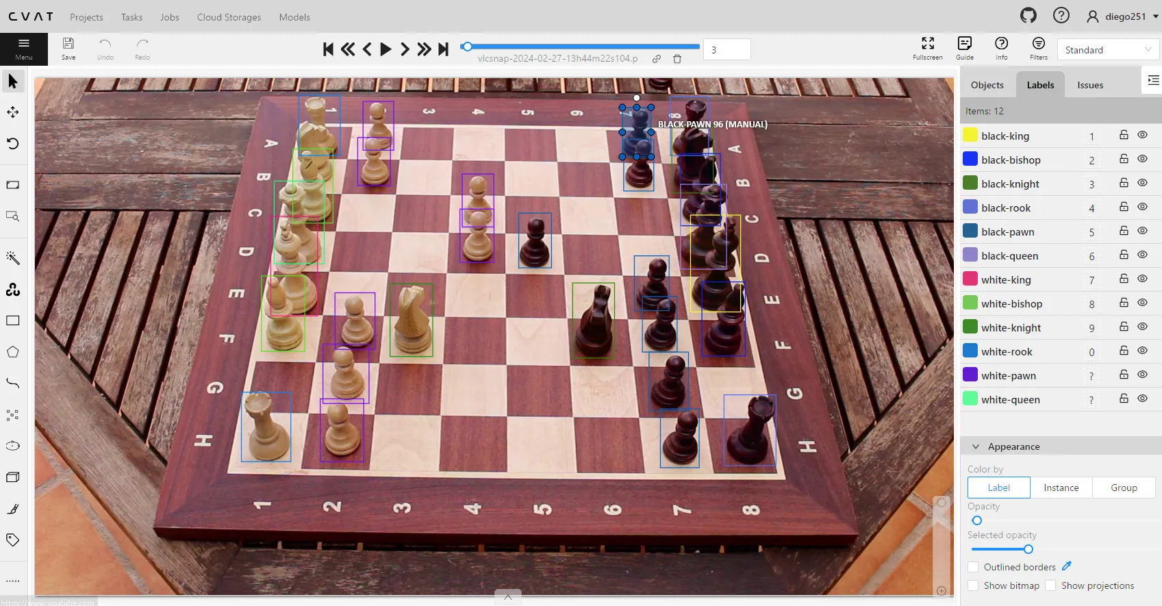
• Labeled using CVAT
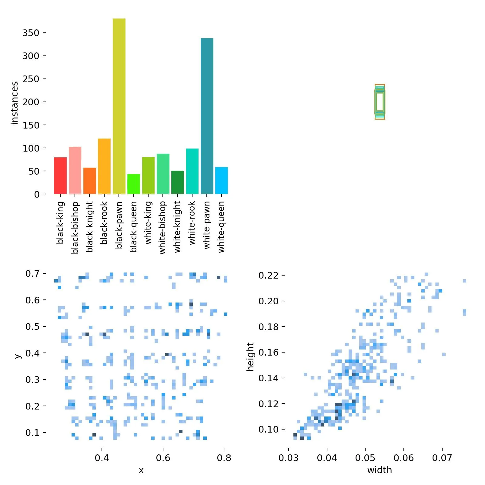
• Distribution:
  • 90 training
  • 30 validation
  • 10 test (never seen during training)

Example label:

// class_id center_x center_y width height
0 0.740893 0.358486 0.054505 0.187343
1 0.750341 0.468051 0.045786 0.155046
1 0.724542 0.215722 0.043604 0.139537
2 0.715820 0.157579 0.045057 0.129194
2 0.762695 0.564556 0.051599 0.144704
// (...)
10 0.339003 0.571662 0.050141 0.114991

Class Index Table

Index	Class Name
0	black-king
1	black-bishop
2	black-knight
3	black-rook
4	black-pawn
5	black-queen
6	white-king
7	white-bishop
8	white-knight
9	white-rook
10	white-pawn
11	white-queen

References

For dataset labeling and move selection, the following sources were referenced for notable chess positions and games:

• My 60 Memorable Games by Bobby Fischer
• Top 10 best chess games of all time!

These resources provided a diverse set of strategic examples to enhance the dataset’s variety and realism.

---

🧠 Piece Classification

Model: YOLOv8 (via Ultralytics)

Training config:

model.train(
  data='dataset.yaml',
  epochs=30,
  batch=-1,
  lr0=0.0001,
  lrf=0.01,
  plots=True
)

Hardware: NVIDIA Tesla T4 (via Google Colab)

Validation: 5-fold cross-validation

📽️ Video Demostration

Chess pieces detection with #YoloV8 for my Final Degree Project: pic.twitter.com/H4aqdLVzcO

— Deinigu (@DeiniguDev) March 11, 2024

♟️ Board Detection

Several classical algorithms were tested:

Algorithm	Result
findChessboardCorners (OpenCV)	❌ Detected only 6x6 boards
Harris / Shi-Tomasi	❌ Noise from surrounding edges
Canny + Hough Transform	✅ Final choice

✅ Final Approach

# Canny edge detection with automatic threshold
def canny_edge(img, sigma=0.33):
  v = np.median(img)
  lower = int(max(0, (1.0 - sigma) * v))
  upper = int(min(255, (1.0 + sigma) * v))
  return cv2.Canny(img, lower, upper)

# Hough line detection
cv2.HoughLines(image, 1, np.pi / 180, 125)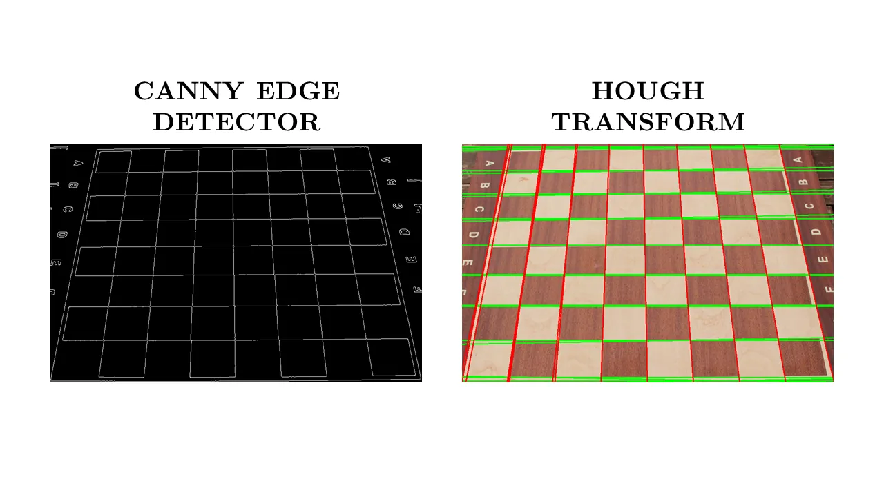

---

✨ Application Flow

The core of the application follows a multi-stage pipeline that combines deep learning with classical computer vision to generate an accurate digital representation of a real chessboard.

Step-by-Step Flow

1. Model Loading

   • Load a pretrained YOLOv8 model (model.pt).
   • If the model is not found, the system stops with a clear error message.

2. Image Input & Validation

   • Accept a .jpg, .jpeg, or .png image via CLI.
   • Ensure the image is tightly cropped around the board.

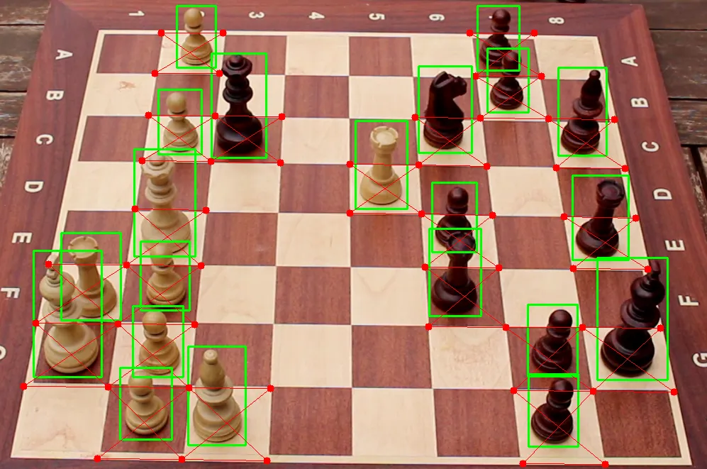
3. Piece Detection & Classification

   • YOLOv8 detects and classifies all pieces.
   • Output saved as labels.txt with piece type, confidence, and bounding box info. For example:

7 0.393105 0.665913 0.0514038 0.158451
9 0.280013 0.47629 0.0551658 0.142217
11 0.345507 0.358007 0.0563328 0.174681
2 0.595982 0.213026 0.0486311 0.138532
5 0.412208 0.203345 0.0514366 0.171442
4 0.652038 0.165326 0.0362755 0.101061
0 0.76361 0.540985 0.0635183 0.19865
6 0.260062 0.534434 0.0618882 0.201384
4 0.693028 0.690002 0.0452681 0.115042
10 0.346834 0.475197 0.0442602 0.108371
10 0.330178 0.676344 0.0461226 0.11515
9 0.53991 0.299925 0.0464019 0.141713
1 0.719523 0.215075 0.0452726 0.143501
10 0.359922 0.230664 0.0392281 0.101181
4 0.60468 0.384311 0.0422276 0.113551
10 0.340781 0.578749 0.0442157 0.112926
4 0.692592 0.57734 0.0440464 0.117031
10 0.374617 0.0966979 0.0360764 0.097045
3 0.73503 0.382123 0.0478531 0.13469
4 0.643071 0.0976982 0.0354422 0.0950123
3 0.605947 0.469218 0.0467537 0.142844

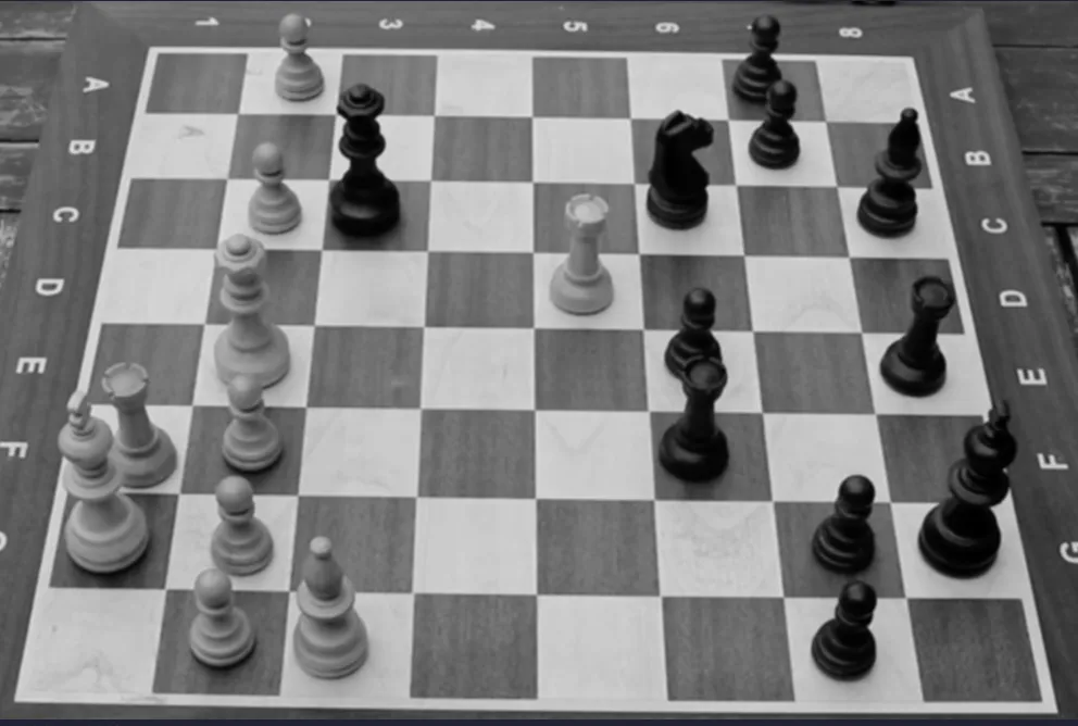
4. Preprocessing

   • Convert image to grayscale.

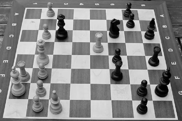
   • Apply Gaussian blur to reduce noise.

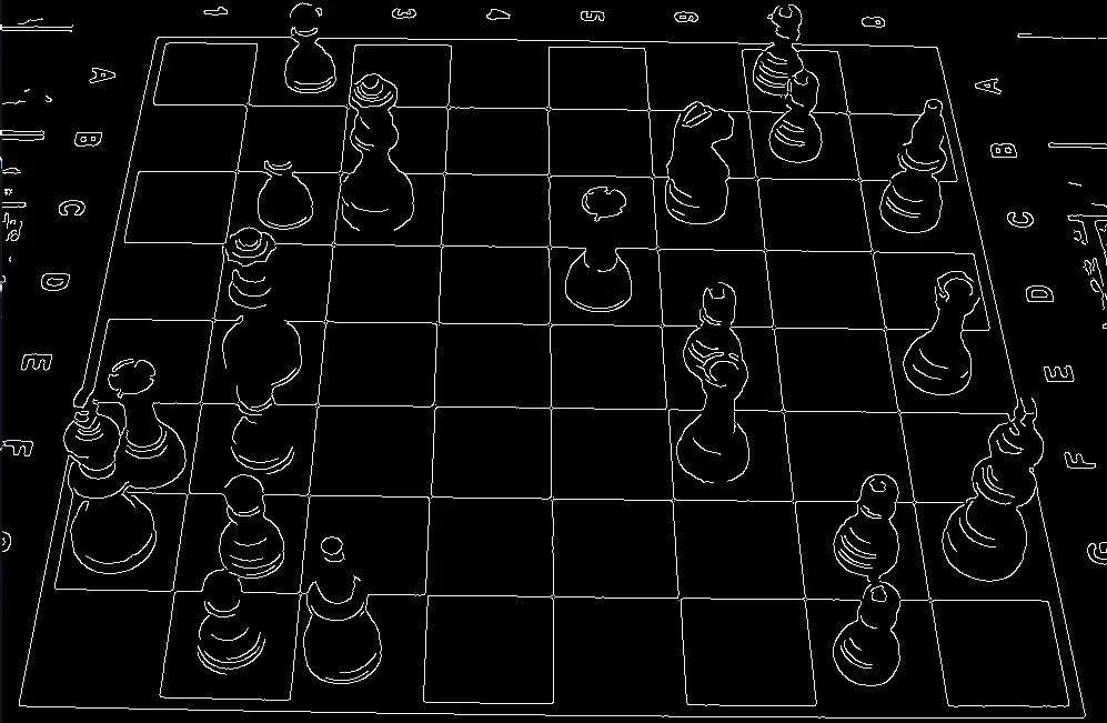
   • Detect edges using Canny edge detector.

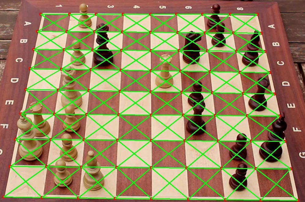
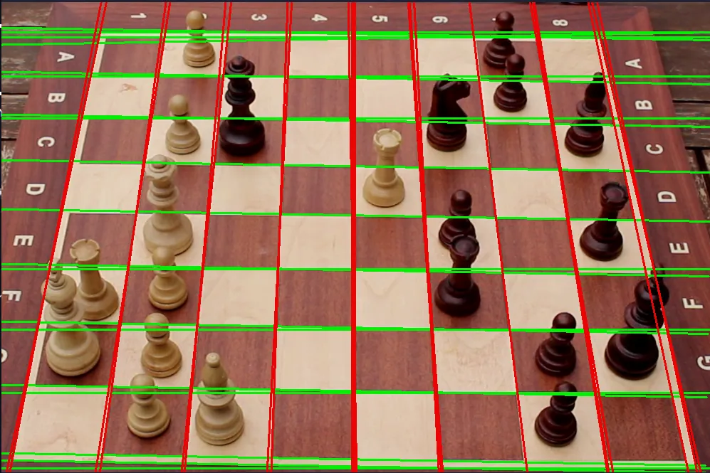
5. Line & Corner Detection

   • Apply Hough Line Transform to detect vertical and horizontal lines.

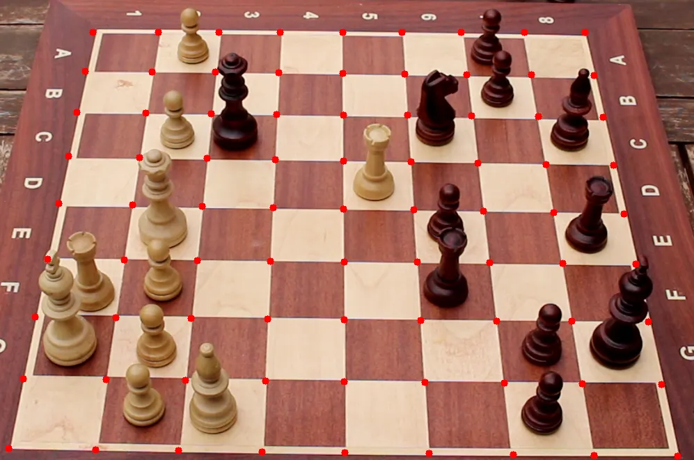
   • Calculate intersections = cell corners.

6. Cell Grid Construction

   • Group intersection points to reconstruct the 8x8 chessboard grid.
   • Assign each cell a board coordinate (e.g., e4, d5).

7. Piece-to-Cell Assignment

   • Match detected bounding boxes to nearest cell center.
   • Handle unassigned pieces using a column-shift strategy.

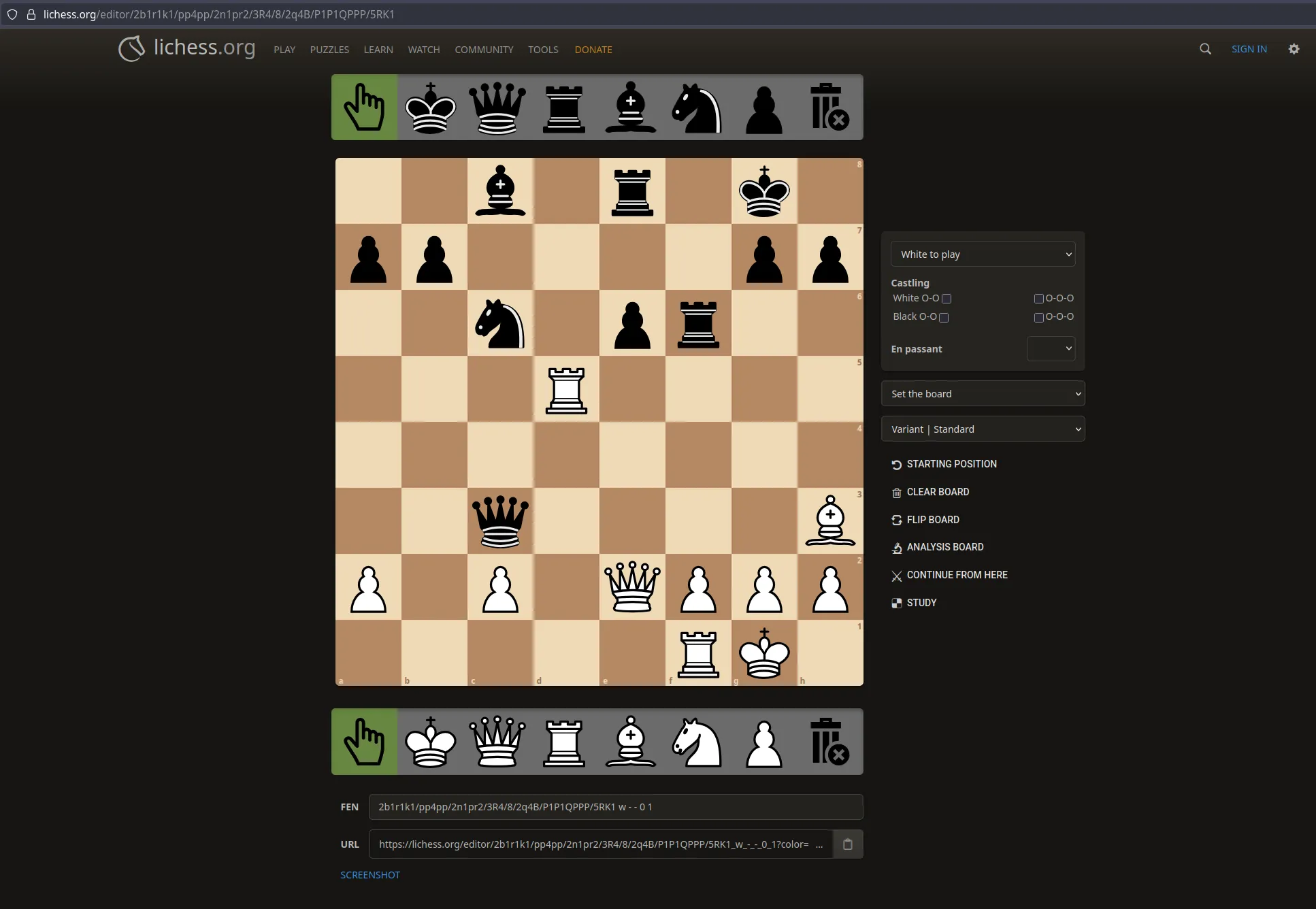
8. FEN Generation

   • Build a FEN string from the final board state.
   • Save FEN to a .txt file and display a Lichess URL with the position.

   2b1r1k1/pp4pp/2n1pr2/3R4/8/2q4B/P1P1QPPP/5RK1

9. Annotated Output

   • Generate images showing:
     • Edge detection
     • Grid overlay
     • Final piece positions
   • Save all images in a timestamped results folder.

10. Debug Mode

    • Optional flag --debug shows intermediate images (grayscale, edges, etc.)

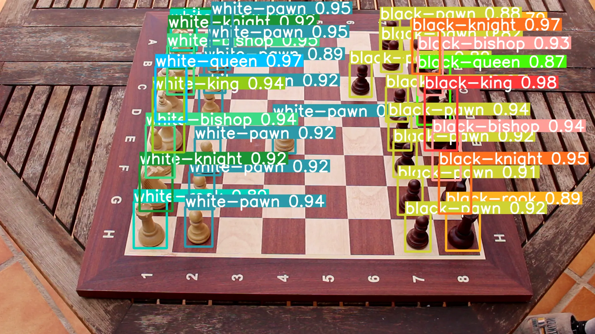
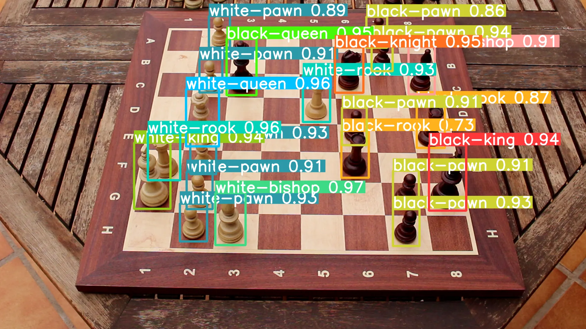
📸 Examples

Example Console Output

❯ python main.py -i workspace/images/test4.png
Model loaded: workspace/model/model.pt

image 1/1 /home/deltablade/TFG-Diego/workspace/images/test4.png: 448x640 1 black-king, 1 black-bishop, 1 black-knight, 2 black-rooks, 5 black-pawns, 1 black-queen, 1 white-king, 1 white-bishop, 2 white-rooks, 5 white-pawns, 2 white-queens, 75.0ms
Speed: 1.1ms preprocess, 75.0ms inference, 187.6ms postprocess per image at shape (1, 3, 448, 640)
Results saved to workspace/results/2025-07-29_15-03-06_test4/predict
1 label saved to workspace/results/2025-07-29_15-03-06_test4/predict/labels
Chessboard from the perspective of the image:
▢ ♟ ▢ ▢ ▢ ▢ ♙ ▢
▢ ▢ ▢ ▢ ▢ ▢ ♙ ▢
▢ ♟ ♕ ▢ ▢ ♘ ▢ ♗
▢ ▢ ▢ ▢ ♜ ▢ ▢ ▢
▢ ♛ ▢ ▢ ▢ ♙ ▢ ♖
♜ ♟ ▢ ▢ ▢ ♖ ▢ ▢
♚ ♟ ▢ ▢ ▢ ▢ ♙ ♔
▢ ♟ ♝ ▢ ▢ ▢ ♙ ▢

Final Result:
▢ ▢ ♗ ▢ ♖ ▢ ♔ ▢
♙ ♙ ▢ ▢ ▢ ▢ ♙ ♙
▢ ▢ ♘ ▢ ♙ ♖ ▢ ▢
▢ ▢ ▢ ♜ ▢ ▢ ▢ ▢
▢ ▢ ▢ ▢ ▢ ▢ ▢ ▢
▢ ▢ ♕ ▢ ▢ ▢ ▢ ♝
♟ ▢ ♟ ▢ ♛ ♟ ♟ ♟
▢ ▢ ▢ ▢ ▢ ♜ ♚ ▢

https://lichess.org/editor/2b1r1k1/pp4pp/2n1pr2/3R4/8/2q4B/P1P1QPPP/5RK1

Example Image Output

Lichess Output

📽️ Video Demostration

Final version executed! I'm thrilled with how project turned out. ♟️ #Chess #AI #YoloV8 #OpenCV #SoftwareDevelopment https://t.co/jp0VNBykG1 pic.twitter.com/GgwBZJ79pB

— Deinigu (@DeiniguDev) August 4, 2024

---

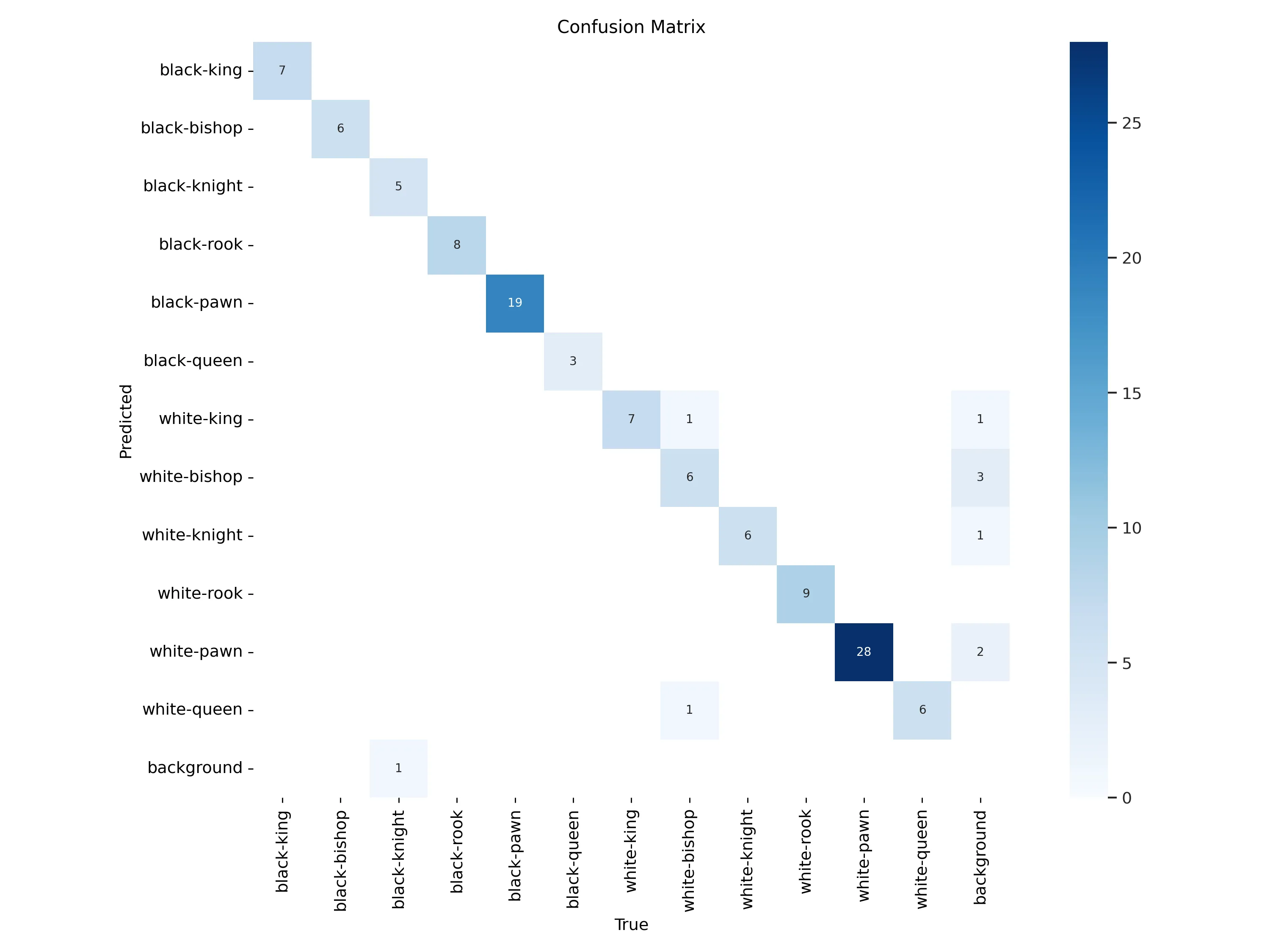
⚗️ Experiments & Evaluation

Two experimental phases were conducted:

📊 Phase 1: Basic Training

• Initial training to test model and pipeline

📈 Phase 2: Cross-Validation

• 5-fold split using .yaml configs
• Averaged metrics for generalization score

for k in range(5):
  model.train(data=ds_yamls[k], ...)
  results[k] = model.metrics

You can find more information in the official paper.

📽️ Video Demostration

As well as that, check out this video showcasing the tests executed! pic.twitter.com/g4CeTXOUjC

— Deinigu (@DeiniguDev) August 4, 2024